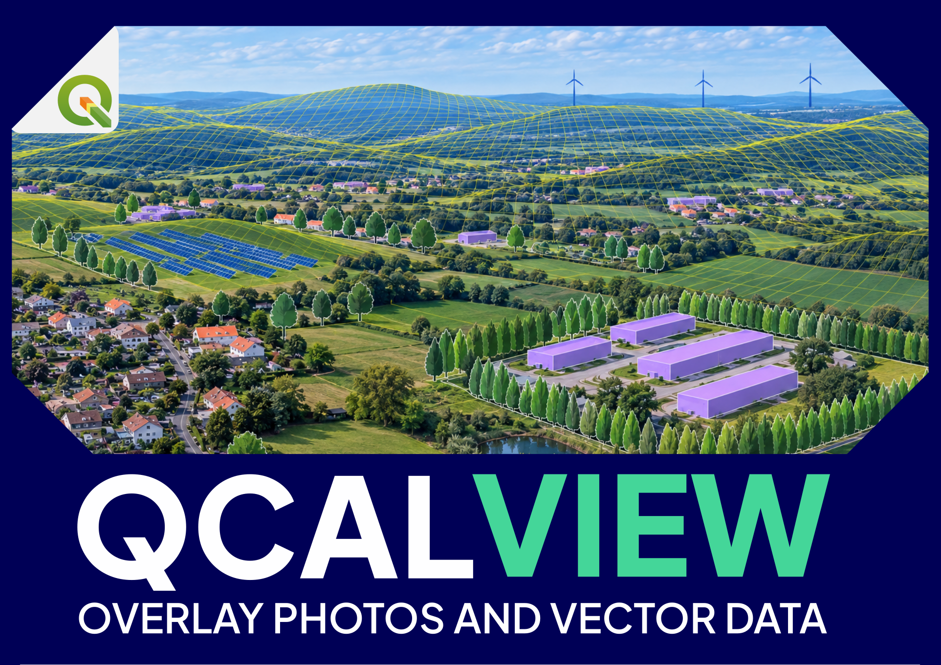
QCALVIEW quick start
Before you start#
Prepare:
- a QGIS project in an appropriate projected CRS;
- a point layer containing one or more viewpoints;
- a terrain raster (DEM/MNT) covering the study area;
- a photograph or panorama for at least one viewpoint;
- one vector layer you can recognize geographically in the scene.
For the first test, choose a photograph with recognizable relief, roads, buildings, turbines, pylons, woodland edges or other mapped features.
Step 1 — Open QCALVIEW and select the viewpoint layer#
Open the QCALVIEW dock and select your viewpoint layer.
QCALVIEW stores camera information in qcv_* fields. If the layer does not yet contain the required fields, let QCALVIEW prepare it rather than manually inventing columns.
Select the current viewpoint.
Step 2 — Assign the photograph#
Associate the image with the viewpoint.
Check that:
- the file is readable;
- its orientation is correct;
- it has already been corrected for significant lens distortion if necessary.
QCALVIEW's PINHOLE model represents an ideal rectilinear camera. Lens distortion is not what the yaw/pitch/FOV controls are intended to fix.
Step 3 — Choose the projection before fine calibration#
Use the projection that matches the image:
- PINHOLE — ordinary rectilinear photograph;
- CYLINDRICAL — cylindrical panorama;
- EQUIRECTANGULAR — 360 × 180 panorama.
A wrong projection cannot usually be repaired by endlessly adjusting FOV or offsets.
Step 4 — Select the DEM#
Select the terrain raster.
Terrain is fundamental for:
- horizon alignment;
- terrain occlusion;
- projected geometry;
- many visibility analyses.
If the terrain is wrong, the apparent calibration may also become wrong.
Step 5 — Calibrate the camera in the right order#
A practical order is:
- viewpoint position;
- projection;
- HFOV / focal length;
- azimuth (yaw);
- pitch;
- roll;
- only then, small image offsets if truly necessary.
Do not use offsets as a substitute for a wrong camera model.
Step 6 — Use terrain and known geometry as evidence#
Display the terrain horizon, ridgelines or a known vector layer.
Ask:
- does the computed horizon follow the photographed skyline?
- do known roads, structures or boundaries project where they should?
- does the fit remain good across the image, not just at the centre?
A calibration that looks correct at one isolated point but drifts elsewhere is usually still wrong.
Step 7 — Project a QGIS layer#
Enable a project layer in QCALVIEW.
You should now see its geometry projected into the calibrated view.
Try:
- a point layer;
- a line or polygon;
- a 2.5D extrusion;
- a schematic motif if applicable.
This is the moment where the value of calibration becomes visible: the GIS layer is no longer just “near” the photograph; it is being drawn through the calibrated camera model.
Step 8 — Save the viewpoint state#
When the calibration and visual state are satisfactory, save the viewpoint state.
This allows QCALVIEW to restore:
- camera parameters;
- image/projection settings;
- relevant visual state;
Step 9 — Create a schematic view#
Switch to schematic view to see that QCALVIEW does not depend on the photograph itself.
The same camera geometry can be used to display terrain and projected data without a photographic background. This is useful for:
- preliminary work before a field visit;
- meetings;
- comparison of project states;
- views for which no photograph is available.
Step 10 — Only then explore analysis and automation#
Start with a simple question such as:
- “How much of this target emerges?”
- “How high must the observer rise before seeing it?”
If the result looks wrong#
Before reporting a rendering problem, check in this order:
- correct CRS and coordinates;
- correct DEM;
- correct projection model;
- correct viewpoint position;
- correct HFOV/VFOV;
- yaw/pitch/roll;
- image distortion/cropping;
- layer visibility and QGIS theme;
- maximum projection distance;
- only then styling and special rendering options.
See the FAQ for common symptoms.