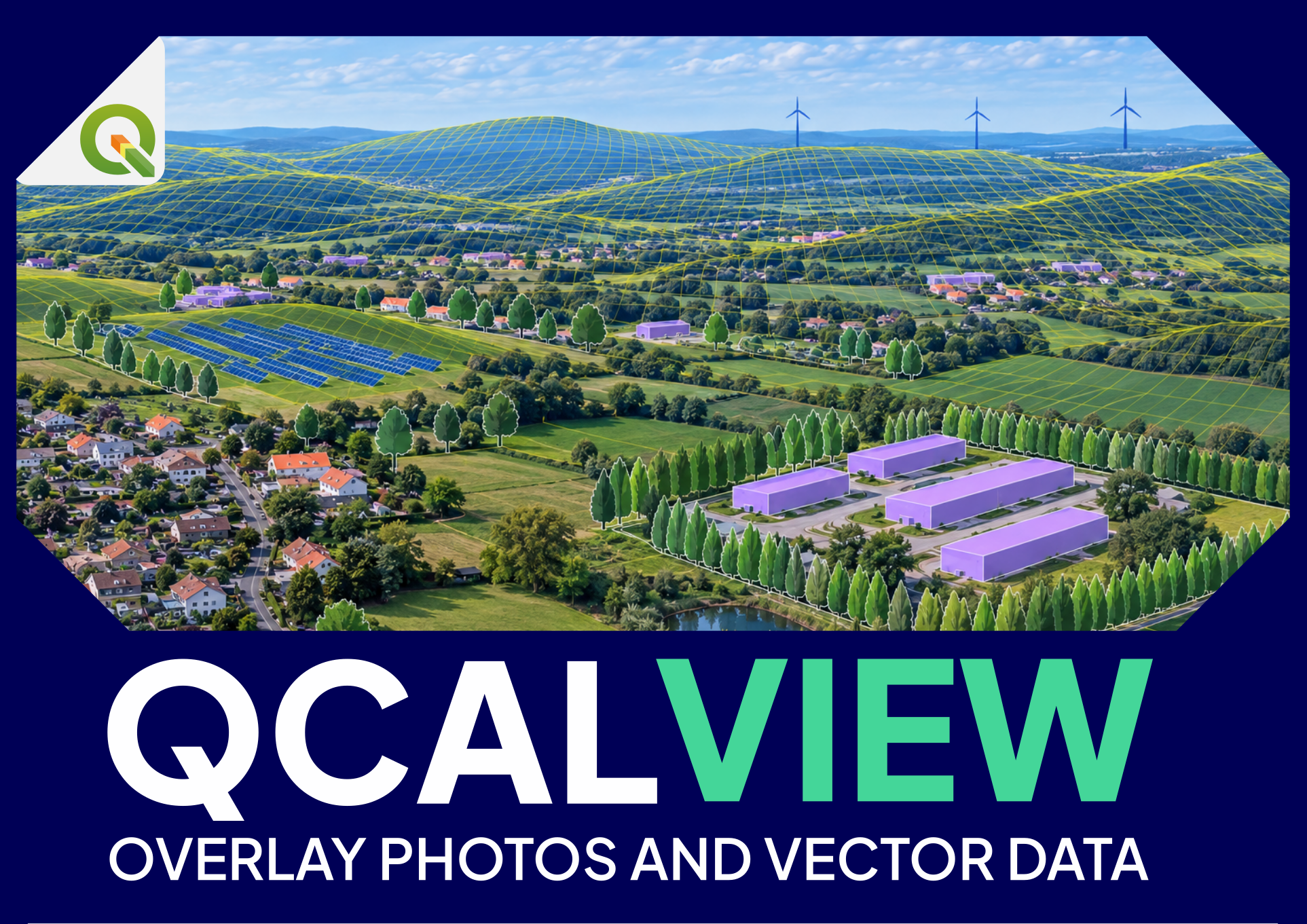
Complete user manual
This manual consolidates the QCALVIEW 40.21 workflow. For deeper explanations, use the dedicated guides linked throughout the page.
1. Purpose and product logic#
QCALVIEW connects five things:
- a geographic viewpoint;
- a camera model;
- terrain;
- QGIS layers;
- optionally, a photograph.
The normal progression is:
CALIBRATE
viewpoint + photograph + camera + terrain
        ↓
VISUALIZE / SIMULATE
project QGIS data, variants, mitigation and schematic states
        ↓
EXPORT / COMMUNICATE
reuse controlled views in the wider project workflow
2. Installation and compatibility#
QCALVIEW 40.21 is designed for the supported QGIS 3.44.x and QGIS 4.x/Qt6 lineages documented by the plugin release.
After installation:
- enable QCALVIEW in QGIS;
- open the QCALVIEW dock;
3. Project coordinate system#
Use a suitable projected CRS for metric work.
A coherent CRS is important for:
- viewpoint/target distances;
- terrain sampling;
- projected geometry;
- screen intersection;
- visibility analysis.
Geographic latitude/longitude layers can be transformed by QGIS, but a local projected work CRS is normally clearer for study distances and debugging.
4. Terrain#
QCALVIEW requires/uses a DEM for most meaningful geographic rendering and visibility calculations.
Terrain supports:
- viewpoint ground elevation;
- horizon calculation;
- terrain occlusion;
- ridgelines;
- raster draping;
- monoplotting;
Choosing a DEM#
Match terrain resolution to the study scale. A high-resolution local study and a 30 km regional study do not have the same needs.
Maximum distance#
Use a realistic maximum projection/analysis distance where appropriate. It reduces unnecessary computation and makes study assumptions explicit.
Earth curvature#
For long-distance work, Earth curvature can become relevant. Keep the setting consistent between analyses that you compare.
5. Viewpoint layer#
A QCALVIEW viewpoint layer is a point layer whose features carry camera/view state through qcv_* attributes.
Typical workflow:
- select the point layer;
- let QCALVIEW prepare required fields;
- select a current viewpoint;
- configure image/camera;
- save the viewpoint state.
Do not casually delete/rename QCALVIEW fields. See Attribute-field reference.
6. Viewpoint identity#
qcv_id is the user-facing identifier.
QCALVIEW may also create qcv_uid, a stable internal identity used to preserve relationships when feature IDs are not stable enough. It is normally hidden and should not be edited manually.
7. Photographs#
The image path is stored in qcv_img.
A source photograph should be:
- available at a stable path;
- in a known projection;
- corrected for significant lens distortion if using PINHOLE;
- understood in terms of crop/stitching.
8. Camera mode and projection#
Photo versus schematic#
A viewpoint can work with a photograph or as a schematic view.
Projection choices#
PINHOLE— ideal rectilinear perspective;CYLINDRICAL— cylindrical panorama;
Choose projection before fine calibration.
9. Camera orientation#
The key orientation parameters are:
qcv_yaw— horizontal direction;qcv_pitch— vertical direction;qcv_roll— rotation about viewing axis.
Use the terrain horizon and known mapped objects rather than adjusting by eye against one feature only.
10. Field of view#
qcv_hfov and qcv_vfov define angular coverage.
Focal length (qcv_foc) and sensor width (qcv_sens) can help derive a rectilinear HFOV, but the final field of view must correspond to the actual image used after crop/stitching/correction.
11. Camera height#
qcv_alt is the camera height/Z parameter. With terrain operation, it normally means observer height above local terrain.
For an eye-level photograph, a value around tripod/eye height may be appropriate. For a drone or elevated platform, use the actual geometric height according to the workflow.
12. Offsets#
qcv_ofh and qcv_ofv provide image offsets, with qcv_ofmd defining their unit mode.
Use offsets as final refinements. Large offsets often indicate a more basic problem with projection, crop, FOV or orientation.
13. Calibration tools#
Terrain horizon / ridgelines#
Use them as geometric references against the photographed skyline.
GCPs#
Use known photo↔map correspondences as control evidence.
Monoplotting#
Click the image to project a viewing ray to the DEM and obtain a geographic point/distance/elevation.
Projection grid / azimuth guide#
Experimental guides can help understand orientation and angular distribution in the image.
See Calibrating a view for the full method.
14. Projected vector layers#
QCALVIEW can project QGIS vector layers through the current camera.
For each layer, think separately about:
- whether it is visible;
- its QGIS style;
- its QCALVIEW representation;
- its physical/schematic height;
- labels;
- terrain occlusion;
- maximum rendering distance.
15. Labels#
Labels may use QGIS label information and/or QCALVIEW display settings depending on the representation.
When labels seem wrong, distinguish:
- label text source;
- label expression;
- text size/style;
- callout/background;
- whether the layer itself is rendered correctly.
16. 2.5D representation#
2.5D is a controlled simplification: 2D vector geometry receives vertical height.
Use it for:
- buildings;
- walls;
- hedges/screens;
- simple project structures;
- explanatory volumes.
17. Schematic motifs#
Schematic motifs provide recognizable visual classes without requiring full 3D models.
Use them to test or communicate:
- vegetation;
- fences;
- agricultural objects;
- repeated linear features;
- simple scene context.
Motif size and geometry should be treated as explicit study assumptions.
18. Raster draping#
QCALVIEW can drape a raster on the terrain and project it into the view.
Possible content:
- visibility classes;
- land cover;
- analysis result;
- constraints;
- project-related rasters.
19. Terrain occlusion#
When enabled, QCALVIEW hides geometry behind terrain according to the DEM.
Remember:
- terrain ≠ vegetation/buildings unless modelled;
- vector screens are a separate explicit model.
20. QGIS map themes#
Map themes are the recommended way to organize visual variants.
Example set:
- Existing;
- Layout A;
- Layout B;
- Layout C;
- With mitigation;
- Mature mitigation.
21. Viewer navigation#
The viewer supports zoom/pan and camera-related interaction.
Use native/100% inspection when pixel-level image work is needed, and fit/zoom views for general coordination.
22. Saving viewpoint state#
Use the explicit save action when you want the current camera/visual state to become the stored state of the viewpoint.
23. Direct export#
Direct QCALVIEW export is the reference interactive export path.
Depending on settings, output may include:
- photograph + overlay;
- schematic view;
- overlay-only PNG.
Keep output framing and dimensions consistent when comparing variants.
24. Why use transparent overlays#
An overlay-only export is useful when:
- a separate layout/compositing tool controls the final image;
- the photographic base must remain untouched;
- you want to compare QCALVIEW geometry against another rendered source.
25. Common troubleshooting: nothing is displayed#
Check:
- layer visibility;
- QGIS theme;
- viewpoint selected;
- DEM selected;
- maximum distance;
- camera direction/FOV;
- projection;
- QCALVIEW representation enabled;
- whether geometry is behind terrain;
- refresh/current-view state.
26. Common troubleshooting: projected layer is misplaced#
Check calibration before styling:
- viewpoint coordinates;
- projection;
- HFOV/VFOV;
- yaw/pitch/roll;
- camera height;
- CRS transformations;
- image crop/distortion.
27. Common troubleshooting: a theme gives unexpected layers#
Separate:
- QGIS theme visibility;
- QCALVIEW saved visual state;
- global/PDV overlays;
Refresh and inspect layer state in QGIS if a toggle/reload changes the result.
28. Common troubleshooting: panorama border artefacts#
Panorama projections have a ±180° seam. QCALVIEW contains special seam handling, but complex 2.5D geometry near the seam is more demanding than ordinary rectilinear rendering.
Confirm the source projection and reproduce with a minimal layer when reporting a problem.
29. Common troubleshooting: calculation is slow#
Reduce/test:
- target count;
- viewpoint count;
- target horizontal samples;
- terrain sampling density;
- distance;
- scenario combinations;
30. Professional study practice#
For any result used externally:
- document source data;
- document camera/viewpoint assumptions;
- keep exact output fields and units;
- preserve detailed tables;
- state analysis bounds;
- visually check representative outputs;
- avoid converting geometric metrics into unsupported qualitative conclusions.
31. Suggested learning path#
First hour#
- calibrate one photograph;
- project one known vector layer;
- save the viewpoint;
- create one schematic view.
Second stage#
- configure 2.5D/motifs;
- create QGIS themes;
- export controlled variants.
Third stage#
- run visibility on one viewpoint × one target;
- inspect fields;
- produce a small map-ready point layer;
- only then scale up.